
User Tools
Sidebar
qcl:simulation_output
This is an old revision of the document!
Table of Contents
Simulation output
For each simulation run, a new output folder is created in the simulation output folder. The created folder has the name of the input file.
In addition, date-time can be added to the folder name by the nextnanomat setting (Tools → Options → Expert settings before Aug 2021, Tools → Options → View/Output since Aug 2021). For nextnanomat before Aug 2021, this option is recommended in order to avoid overwriting existing output data. For nextnanomat after Aug 2021, simulation output is per default not overwritten and instead enumerated unless you manually check the option “Overwrite existing simulation…”.
The created output folder contains:
- the input file (.xml) and the material database (.xml).
- a folder 'Input' which contains material parameters used in the calculation.
- a folder Strain (only if the strain option is activated).
- a folder Polarization if pyroelectric and/or piezoelectric effects are considered.
- a folder 'Init_Electron_Modes' for the results of the initial Schrödinger solution.
- a folder for each parameter step. In particular, in case of voltage sweep, the name of the folder is the potential drop per period.
- Several files related to the sweep made. For a voltage sweep, it contains plots of physical quantities (current, gain,…) as a function of the applied voltage.
- a log file is created at the end of the simulation, containing all the information displayed during the simulation.
'Input' folder
The folder Input/ contains all the simulation input such as material parameters as a function of position.
AlloyContent.dat
alloy concentration $x$ vs. position for ternary materials such asAl(x)Ga(1-x)AsAlloyScatteringTerm.dat
alloy scattering term (in unit of [eV$^2$]) vs. position for ternary materialsBandEdges.dat
conduction band edge $E_{\rm c}$ and valence band edge $E_{\rm v}$ vs. position in units of [eV]BandGap.dat
energy band gap $E_{\rm gap}$ vs. position in units of [eV]Conduction_BandEdge.dat
conduction band edge $E_{\rm c}$ including shift due to strain vs. position in units of [eV]DeformationPotential_ConductionBand.dat
conduction band deformation potential vs. positionDeformationPotential_ValenceBand.dat
valence band deformation potential vs. positionDeformationPotential_ValenceBand_Uniaxial.dat
valence band uniaxial deformation potential vs. positionDopingDensity.dat
Doping density [cm$^{-3}$] vs. positionE_p(Kane energy).dat
Kane energy [eV] (material-dependent k.p parameter) vs. positionEffectiveMass.dat
effective conduction band mass $m_{\rm c}$ vs. position in units of [m0]. This input is not used for a k.p calculation.ElasticConstants.dat
elastic constants $c_{ij}$ vs. position in units of [GPa]EpsOptic.dat
optical dielectric constant $\epsilon(\infty)$ vs. positionEpsStatic.dat
static dielectric constants $\epsilon(0)$ vs. positionL (Dresselhaus parameter L).dat
Dresselhaus parameter (material-dependent k.p parameter) vs. position. Default is $-1$.LatticeConstants.dat
lattice constants $a$ vs. position in units of [nm]MaterialDensity.dat
material density vs. position in units of [kg/m3]PhononEnergy_LO.dat
longitudinal optical (LO) phonon energy in units of [eV]PiezoConstants.dat
piezoelectric constants $e_{ij}$ in units of [C/m2]PyroConstants.dat
pyroelectric polarization $P_z$ (spontaneous polarization) in units of [C/m2] (wurtzite only)S (remote band parameter).dat
remote band parameter (material-dependent k.p parameter) vs. positionVelocityOfSound.dat
sound velocity in units of [m/s]
Strain
If the strain option is activated, a folder Strain/ is created.
Strain_CrystalSystem.dat
(dimensionless) strain tensor components with respect to the crystal coordinate system.Strain_Simulation.dat
(dimensionless) strain tensor components with respect to the simulation coordinate system.
If the crystal has not been rotated, above files contain identical values.
Strain_trace.dat
trace of the strain tensor
Piezo and pyroelectric polarization
The folder Polarization/ contains the piezoelectric and pyroelectric polarization if these options are activated.
InterfaceCharges\PiezoCharges.dat
piezoelectric charge density due to strain. If the strain is zero, the piezoelectric charge density is zero.InterfaceCharges\PyroCharges.dat
pyroelectric charge density due to spontaneous polarization in wurtzite crystals.PiezoPolarization.dat
$z$-component of the piezoelectric polarization vectorPyroPolarization.dat
$z$-component of the pyroelectric polarization vector
Initial electronic states
The folder Init_Electr_Modes\ contains 3 different folders corresponding to 3 different sets of basis states. They are calculated at the first step of the calculation, before the NEGF calculation. These 3 sets of states are basis of the reduced Hilbert space obtained after applying the energy cut-off <Energy_Range_Axial>.
These states are displayed for a default voltage of <Energy_Range_Axial>/2. This voltage at which the states are visualized can be modified by the input file command:
<Simulation_Parameter>
  ...
  <Bias_for_initial_Electronic_Modes unit="meV">54</Bias_for_initial_Electronic_Modes>
  ...
</Simulation_Parameter>
'Reduced Real Space' modes
The 'reduced real space' modes are eigenstates of the position operator in the reduced Hilbert space (i.e. after the energy cut-off). Because of the energy cut-off, these states are spatially extended instead of being $\delta$ functions. This basis set is the one which is used in the NEGF calculation. It does not depend on the applied voltage. However, this basis has generally little use in terms of physical interpretation.
The folder Init_Electr_Modes\ReducedRealSpace\ contains:
ReducedRealSpaceModes.dat
Conduction band edge and square of the wave functions (shifted in energy) vs. the heterostructure coordinate position.
3 periods are displayed. (p0) means period 0 (left period), (p1) means period 1 (central period), and p2 period 2 (right period). The numbers of states displayed is equal to 3 times the number of states per period, that is the number of selected minibands.

ReducedRealSpaceModesOn.dat
Same as inReducedRealSpaceModes.datbut the vanishing parts of the wavefunctions are not shown (plot not supported by nextnanomat).H0ReducedRealSpace_nobias.mat
Expression of the Hamiltonian in this basis when no external bias voltage is applied.H0ReducedRealSpace_nobias.mat
Expression of the Hamiltonian in this basis with an applied external voltage.- Single-band case:
Wavefunction.dat
Envelope function of the wavefunction $\Psi_i(z)$ - Multiband-case:
Wavefunction_ConductionBand.dat,Wavefunction_LHBand.dat, andWavefunction_SOBand.dat
Different component of the envelope wavefuntions
$$\Psi_i(z) = f^{\text{c}}_i(z)u_{\text{c}}(z) + f^{\text{LH}}_i(z)u_{\text{LH}}(z) + f^{\text{SO}}_i(z)u_{\text{SO}}(z)$$
'Tight-binding' states
The Tight-binding\ folder contains data only if one or several <Analysis_Separator> are defined in the input file. The tight-binding basis corresponds to piecewise solution of the Schrödinger equation between these separators.

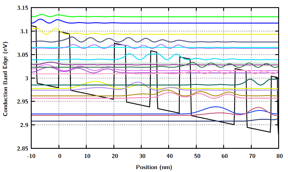
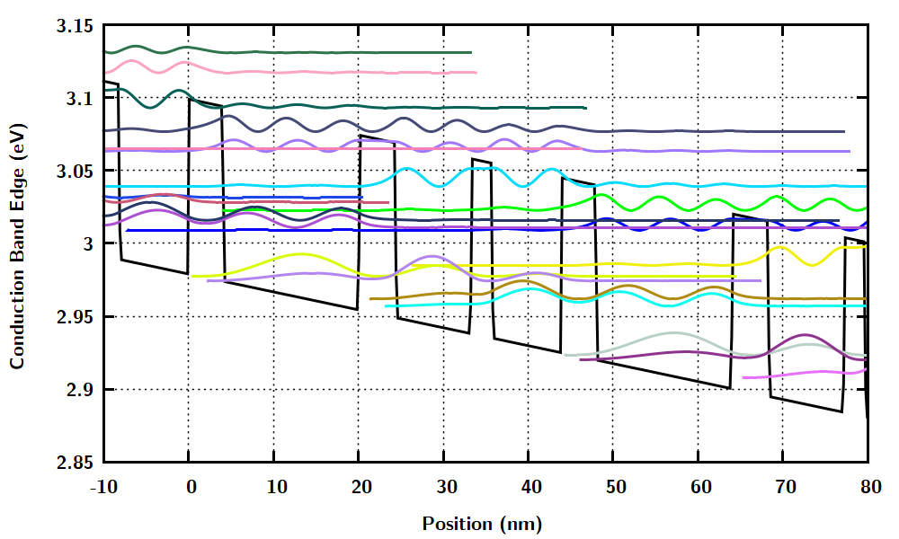
Wannier-Stark states
The Wannier-Stark states correspond to the eigenstates of the Schrödinger equation without accounting for Poisson equation (i.e. electrostatic mean-field).
It contains:
Wannier-Stark_States.datshows the conduction band edge and the probability densities of the eigenstates of the Wannier-Stark states. Schrödinger equation.
Wannier-Stark_levelsOn.dat. Same asWannier-Stark_States.datexcept that the points with almost zero probability density are omitted.
Dipoles.matgives the dipole matrix elements (i.e. matrix elements of the position operator)
The expression in the single-band case is: $$ d_{ij} = \int dz f_i(z) ~ z ~ f_j(z) $$ In the multiband case: $$ d_{ij} = \sum_{\mu} \int dz f^{(\mu)}_i(z) ~ z ~ f^{(\mu)}_j(z) $$
EffectiveMasses.datgives the position and energy-dependent effective massH0_WannierStark.matgives the Hamiltonian in the Wannier-Stark basis.Oscillator_Strength.matgives the oscillator strengths.
In-plane discretization
The file Lateral_spectrum.dat gives the energy discretization for the states used to describe the 2-Dimensional (2D) motion in the directions (x,y) perpendicular to the heterostructure. The lateral motion is discretized using cylindrical boundary conditions, and the corresponding eigenstates are Bessel funcitons.
$x$ axis: Lateral state index
$y$ axis: order of Bessel (zero index)-1 of Bessel Relative Energy (meV).
Simulation output for each voltage/temperature step
For each voltage or temperature step, the following files are produced as a result of the NEGF calculation:
CarrierDensity.dat
Electron density in [cm-3] as a function of position [nm].
Conduction_BandEdge.dat
Calculated heterostructure conduction band edge profile $E_{\rm c}^\prime$ as a function of position in units of [eV]. It includes the mean field electrostatic potential $\phi$ [V] as $E_{\rm c}^\prime = E_{\rm c} - e \phi$.
Convergence.txt
This file contains values for- Convergence factor
convergence factor for the lesser Green's function $\mathbf{G}^<$, which corresponds to the relative variation between the last two consecutive Green's functions. Should be as close as possible to 0. - Current convergence factor
convergence factor for the current density, which corresponds to the relative variation of the last two consecutive current density values. Should be as close as possible to 0. - Number of iterations
- Normalization of lesser Green's function $\mathbf{G}^<$
Should be as close as possible to 1. - Sum normalised spectral function
Should be as close as possible to 1. If not, it usually means that the energy grid spacing is too large.
NO-CONVERGENCE.txt
This file is generated instead if the calculation did not converge.
CurrentDensity.dat
Current density in [A/cm2] as a function of position [nm].
Current-miscellaneous.txt
General information on the simulation.- Current density in [A/cm2]
- Average electron velocity in [nm/ps]
- Time for one electron to travel through one period in [ps]
- Electric field in [kV/cm]
- Doping sheet density per period in [cm-2]
- 3D doping density averaged over one period in [cm-3]
- Effective electronic temperature in [Kelvin]. This is only an effective temperature as electrons are not in thermal equilibrium, which is obtained by averaging the kinetic energy for the in-plane motion. This effective temperature is given by the following formula:
$$ T_{\text{eff}} = \sum_{i} ~ p_{i} ~ E_{\parallel}(i) ~ / ~ k_b $$ where $p_{i}$ is the fraction (i.e. population normalized to 1) of occupation in the in-plane state $i$, $E_{\parallel}(i)$ is the in-plane energy for the in-plane state $i$, and k_b the Boltzmann constant.
Electrostatic-Potential.dat
Mean field electrostatic potential $\phi$ [V] as a function of position. The electrostatic potential $\phi$ is the solution of the Poisson equation and has been calculated self-consistently.
Output in basis sets (ReducedRealSpace, WannierStark, TightBinding)
3 folders are created to output physical quantities in the 3 different basis sets (Reduced Real Space, Wannier-Stark, and Tight-Binding).
For each basis set, the folder contains:
- the probability density $\vert \Psi_i(z) \vert^2$ for the each state $\Psi_i$. Each level is shifted accordingly to its energy.
- the wavefunction $\Psi_i(z)$ in the file
Wavefunctions.dat CarrierDistribution_Energy.datshows the energy-resolved populations in each state.DensityMatrix.txtdisplays the density matrix in a text file.DensityMatrix_Real.matdisplays the real part of the density matrix. The labeling is made accordingly to the one of the wavefunctions $\Psi_i(z)$, so that the matrix element (i,j) corresponds to the real part of $\langle \Psi_i \vert \rho \vert \Psi_j \rangle$, where $\rho$ is the density matrix. Note that the diagonal element (i,i) is equal to the population of the level $\Psi_i$.DensityMatrix_Imaginary.matdisplays the imaginary part of the density matrix.Dipoles.matgives the dipole matrix elements (see above for definition)EffectiveMasses.datgives the position and energy-dependent effective massPopulations.textindicates the population (i.e. the probability of occupation) in each level $\Psi_i$ (normalized to 1 for one period of the structure).SpectralFunctions.datshows the diagonal part of the spectral function, i.e. the energy-resolved density of states (DOS).Subband_KineticEnergy.txtcontains the averaged kinetic energy for each level/subband $i$. Its calculation is given by:
$$ \langle E_i \rangle = \frac{ \sum_{k} ~ p_{i,k} ~ E_{\parallel}(k)}{\sum_{k} ~ p_{i,k}} $$, where $E_{\parallel}(k)$ is the in-plane kinetic energy.
Subband_Temperature.txtgives the effective temperature of each level/subband $i$, according to
$$ T^{\text{eff}}_i = \langle E_i \rangle / ~ k_b $$
2D plots
The folder 2D_Plots_Position-nm_Energy-eV/ contains files where the $x$ axis is position in [nm] and the $y$ axis is energy in units of [eV].
Note that these 2D plots show 2 QCL periods although only 1 period is simulated.
DOS_energy_resolved.vtr/*.gnu/*.fld
This file contains the energy-resolved local density of states ${\rm LDOS}(x,E)$ as a function of position and energy. The units are [eV-1 nm-1]).
The local density of states is related to the spectral function. It shows the available states for the electrons at $k_\parallel = 0$.
CarrierDensity_energy_resolved.vtr/*.gnu/*.fld
This file contains the energy-resolved electron density $n(x,E)$ as a function of position and energy. The units are [cm-3 eV-1]. The energy-resolved electron density is related to the Green's function $\mathbf{G}^<$ (“G lesser”).CurrentDensity_energy_resolved.vtr/*.gnu/*.fld
This file contains the energy-resolved current density $j(x,E)$ as a function of position and energy. The units are [A cm-2 eV-1].
Gain
The folder Gain/ contains files where the $x$ axis is position in [nm] and the $y$ axis is photon energy $E_{\rm ph}$ in units of [eV].
Note that these 2D plots show 2 QCL periods although only 1 period is simulated.
Energy-Resolved_Gain_Simple-Approximation.fld/*.coord/*.dat
This file contains the energy-resolved intensity gain $G(x,E_{\rm ph})$ as a function of position and photon energy $E_{\rm ph}$. The units are [cm-1 nm-1]. (Note that the units of the nextnano.MSB code are [eV-1 cm-1].
Gain_Simple-Approximation.dat
This file contains the gain obtained without the self-consistent calculation.
The $x$ axis is energy in units of [meV].
The $y$ axis is the gain in units of [1/cm]. A negative value of gain corresponds to absorption.
Gain_SelfConsistent.dat
This file contains the intensity gain obtained with the self-consistent calculation.
The $x$ axis is energy in units of [meV].
The $y$ axis is the gain in units of [1/cm].
A negative value of gain corresponds to absorption.
Note that the gain output is only done for the voltages specified in the input file.
<!-- Calculate gain only between the following values of
     potential drop per period in order to save CPU time -->
     <Vmin unit="mV"> 160 </Vmin>
     <Vmax unit="mV"> 400 </Vmax>
Green's functions
The folder GreenFunctions/ contains information on the Green's functions.
The electron density $n(x,E_x)$ is related to the lesser Green's function $\mathbf{G}^<$ (“G lesser”): $$n(x,E_x) = - \frac{{\rm i}}{2\pi} \mathbf{G}(x,x^\prime=x,E_x)$$
GreenLesser_All.dat
lesser Green's function $\mathbf{G}^<$
This file contains the sum over all the diagonal (i.e. $x=x^\prime$) lesser Green's functions (sum over one period) as a function of energy $E_x$.GreenLesser_Z.dat
lesser Green's function $\mathbf{G}^<$
This file contains the lesser Green's function $\mathbf{G}^<$ (i.e. density $n(E)$) for each mode space used in the calculation.
The local density of states $\rho(x,E_x)$ is related to the spectral function $\mathbf{A}$: $$\rho(x,E_x) = \frac{1}{2\pi} \mathbf{A}(x,x^\prime=x,E_x)$$ $\mathbf{A}$ is defined as $\mathbf{A} = {\rm i} (\mathbf{G}^{\rm R} - \mathbf{G}^{{\rm R}\dagger}) = - 2 {\rm Im}(\mathbf{G}^{\rm R})$. $\mathbf{G}^{\rm R}$ is the retarded Green's function.
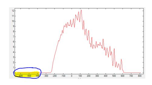
GreenSpectral_All.dat
This file contains the sum over all the spectral functions (sum over one period) as a function of energy $E_x$.
Example: In the figure below, for instance, one can see that<Emin_shift unit="meV">can be increased (by 200 meV) to reduce the calculation time. Essentially, the energy range of the Green's functions is altered by adjusting<Emin_shift unit=meV>and<Emax_shift unit=meV>.

GreenSpectral_Z.dat
This file contains the spectral function for each mode space used in the calculation.
Density matrix
The folder DensityMatrix/ contains the density matrix $\rho$ which is a complex quantity and it is dimensionless.
The trace of the density matrix equals 1.
In our case, the trace is 1 if we sum over one period.
The state labels (state $i$, period $j$) are specified in the complex density matrix.
$$\rho(i,j) = \rho({\rm state},{\rm period})$$
DensityMatrix_complex.mat
This file contains the density matrix.
The $x$ axis contains real and imaginary value.
The $y$ axis is number of periods.DensityMatrix_RealPart_AbsoluteValue.mat
This file contains the absolute value of the real part of the density matrix.
The $x$ axis contains absolute value of the imaginary part.
The $y$ axis is number of periods.DensityMatrix_ImaginaryPart_AbsoluteValue.mat
This file contains the absolute value of the imaginary part of the density matrix.
The $x$ axis contains absolute value of the real part.
The $y$ axis is number of periods.
Output files for voltage sweep
For each simulation, the following files are produced.
Energy_WannierStarkStates.dat
This file contains the energy levels of the Wannier-Stark states (“E_1 = Energy of level 1”, “E_2 = Energy of level 2”,…) as a function of voltage, i.e. potential drop per period in units of [mV].Gain_vs_Voltage.datandGain_vs_EField.dat
These files contain the intensity gain as a function of voltage or electric field respectively.
The $x$ axis is the potential drop per period [mV] (or electric field [kV/cm]).
The $y$ axis contains the maximum gain in [1/cm] and the photon energy for maximum gain [meV] (or photon frequency in [THz]).0Current_vs_Voltage.datandCurrent_vs_EField.dat
These files contain current-voltage characteristics, i.e. the current density in units of [A/cm2] as a function of voltage (i.e. potential drop per period in units of [mV]) or electrif field in [kV/cm]. The current is the average of the fileCurrent-Density.dat.
Combined temperature-voltage sweep
a combined temperature-voltage sweep can be done using the keyword Temperature-Voltage in the field <SweepType> of <SweepParameters> (see the example of code below). In this case, the simulation can be parallelized. <Threads> defines the number of parallel threads. Its optimal value should be the number of CPU cores available (if the available memory is sufficient). Within each parallel temperature sweep, a serial voltage sweep is performed.
<SweepParameters>
    <SweepType>Temperature-Voltage</SweepType>
    <MinV> 50</MinV>
    <MaxV> 60</MaxV>
    <DeltaV> 2</DeltaV>

    <MinT> 25</MinT>
    <MaxT> 300</MaxT>
    <DeltaT> 25</DeltaT>

    <Threads>12</Threads> <!-- Parallelization for Temperature-Voltage sweep -->
</SweepParameters>
Note that for such voltage-temperature sweep, <Maximum_Number_of_Threads> in <Simulation_Parameter> should be set to 1. (A combined parallelization will result in lower performances.)
<Simulation_Parameter>
  ...
  <Maximum_Number_of_Threads>1</Maximum_Number_of_Threads>
</Simulation_Parameter>
At the end of the simulation, current and gain maps can be displayed.
Gain_map.fld gives the maximum gain at each (voltage,temperature) point.
Max_Gain_frequency.fld gives the map of the corresponding photon energy for which the gain is maximum.
Folder view:

Gain map (V,T):

qcl/simulation_output.1629292938.txt.gz · Last modified: 2021/08/18 13:22 by takuma.sato